Recursion

Hello recursion!

We mention recursion briefly in the previous chapter. In this chapter, we’ll take a closer look at recursion, why it’s important to Haskell and how we can work out very concise and elegant solutions to problems by thinking recursively.

If you still don’t know what recursion is, read this sentence. Haha! Just kidding! Recursion is actually a way of defining functions in which the function is applied inside its own definition. Definitions in mathematics are often given recursively. For instance, the fibonacci sequence is defined recursively. First, we define the first two fibonacci numbers non-recursively. We say that F(0) = 0 and F(1) = 1, meaning that the 0th and 1st fibonacci numbers are 0 and 1, respectively. Then we say that for any other natural number, that fibonacci number is the sum of the previous two fibonacci numbers. So F(n) = F(n-1) + F(n-2). That way, F(3) is F(2) + F(1), which is (F(1) + F(0)) + F(1). Because we’ve now come down to only non-recursively defined fibonacci numbers, we can safely say that F(3) is 2. Having an element or two in a recursion definition defined non-recursively (like F(0) and F(1) here) is also called the edge condition and is important if you want your recursive function to terminate. If we hadn’t defined F(0) and F(1) non recursively, you’d never get a solution any number because you’d reach 0 and then you’d go into negative numbers. All of a sudden, you’d be saying that F(-2000) is F(-2001) + F(-2002) and there still wouldn’t be an end in sight!

Recursion is important to Haskell because unlike imperative languages, you do computations in Haskell by declaring what something is instead of declaring how you get it. That’s why there are no while loops or for loops in Haskell and instead we many times have to use recursion to declare what something is.

Maximum awesome

The maximum function takes a list of things that can be ordered (e.g. instances of the Ord typeclass) and returns the biggest of them. Think about how you’d implement that in an imperative fashion. You’d probably set up a variable to hold the maximum value so far and then you’d loop through the elements of a list and if an element is bigger than then the current maximum value, you’d replace it with that element. The maximum value that remains at the end is the result. Whew! That’s quite a lot of words to describe such a simple algorithm!

Now let’s see how we’d define it recursively. We could first set up an edge condition and say that the maximum of a singleton list is equal to the only element in it. Then we can say that the maximum of a longer list is the head if the head is bigger than the maximum of the tail. If the maximum of the tail is bigger, well, then it’s the maximum of the tail. That’s it! Now let’s implement that in Haskell.

maximum' :: (Ord a) => [a] -> a
maximum' [] = error "maximum of empty list"
maximum' [x] = x
maximum' (x:xs)
    | x > maxTail = x
    | otherwise = maxTail
    where maxTail = maximum' xs

As you can see, pattern matching goes great with recursion! Most imperative languages don’t have pattern matching so you have to make a lot of if else statements to test for edge conditions. Here, we simply put them out as patterns. So the first edge condition says that if the list is empty, crash! Makes sense because what’s the maximum of an empty list? I don’t know. The second pattern also lays out an edge condition. It says that if it’s the singleton list, just give back the only element.

Now the third pattern is where the action happens. We use pattern matching to split a list into a head and a tail. This is a very common idiom when doing recursion with lists, so get used to it. We use a where binding to define maxTail as the maximum of the rest of the list. Then we check if the head is greater than the maximum of the rest of the list. If it is, we return the head. Otherwise, we return the maximum of the rest of the list.

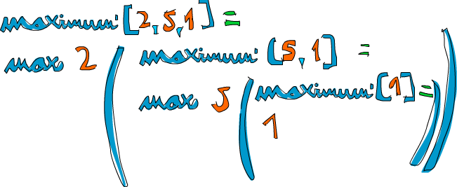
Let’s take an example list of numbers and check out how this would work on them: [2,5,1]. If we call maximum' on that, the first two patterns won’t match. The third one will and the list is split into 2 and [5,1]. The where clause wants to know the maximum of [5,1], so we follow that route. It matches the third pattern again and [5,1] is split into 5 and [1]. Again, the where clause wants to know the maximum of [1]. Because that’s the edge condition, it returns 1. Finally! So going up one step, comparing 5 to the maximum of [1] (which is 1), we obviously get back 5. So now we know that the maximum of [5,1] is 5. We go up one step again where we had 2 and [5,1]. Comparing 2 with the maximum of [5,1], which is 5, we choose 5.

An even clearer way to write this function is to use max. If you remember, max is a function that takes two numbers and returns the bigger of them. Here’s how we could rewrite maximum' by using max:

maximum' :: (Ord a) => [a] -> a
maximum' [] = error "maximum of empty list"
maximum' [x] = x
maximum' (x:xs) = max x (maximum' xs)

How’s that for elegant! In essence, the maximum of a list is the max of the first element and the maximum of the tail.

A few more recursive functions

Now that we know how to generally think recursively, let’s implement a few functions using recursion. First off, we’ll implement replicate. replicate takes an Int and some element and returns a list that has several repetitions of the same element. For instance, replicate 3 5 returns [5,5,5]. Let’s think about the edge condition. My guess is that the edge condition is 0 or less. If we try to replicate something zero times, it should return an empty list. Also for negative numbers, because it doesn’t really make sense.

replicate' :: (Num i, Ord i) => i -> a -> [a]
replicate' n x
    | n <= 0    = []
    | otherwise = x:replicate' (n-1) x

We used guards here instead of patterns because we’re testing for a boolean condition. If n is less than or equal to 0, return an empty list. Otherwise, return a list that has x as the first element and then x replicated n-1 times as the tail. Eventually, the (n-1) part will cause our function to reach the edge condition.

Next up, we’ll implement take. It takes a certain number of elements from a list. For instance, take 3 [5,4,3,2,1] will return [5,4,3]. If we try to take 0 or fewer elements from a list, we get an empty list. Also if we try to take anything from an empty list, we get an empty list. Notice that those are two edge conditions right there. So let’s write that out:

take' :: (Num i, Ord i) => i -> [a] -> [a]
take' n _
    | n <= 0   = []
take' _ []     = []
take' n (x:xs) = x : take' (n-1) xs

The first pattern specifies that if we try to take a 0 or negative number of elements, we get an empty list. Notice that we’re using _ to match the list because we don’t really care what it is in this case. Also notice that we use a guard, but without an otherwise part. That means that if n turns out to be more than 0, the matching will fall through to the next pattern. The second pattern indicates that if we try to take anything from an empty list, we get an empty list. The third pattern breaks the list into a head and a tail. And then we state that taking n elements from a list equals a list that has x as the head and then a list that takes n-1 elements from the tail as a tail. Try using a piece of paper to write down how the evaluation would look like if we try to take, say, 3 from [4,3,2,1].

reverse simply reverses a list. Think about the edge condition. What is it? Come on … it’s the empty list! An empty list reversed equals the empty list itself. O-kay. What about the rest of it? Well, you could say that if we split a list to a head and a tail, the reversed list is equal to the reversed tail and then the head at the end.

reverse' :: [a] -> [a]
reverse' [] = []
reverse' (x:xs) = reverse' xs ++ [x]

There we go!

Because Haskell supports infinite lists, our recursion doesn’t really have to have an edge condition. But if it doesn’t have it, it will either keep churning at something infinitely or produce an infinite data structure, like an infinite list. The good thing about infinite lists though is that we can cut them where we want. repeat takes an element and returns an infinite list that just has that element. A recursive implementation of that is really easy, watch.

repeat' :: a -> [a]
repeat' x = x:repeat' x

Calling repeat 3 will give us a list that starts with 3 and then has an infinite amount of 3’s as a tail. So calling repeat 3 would evaluate like 3:repeat 3, which is 3:(3:repeat 3), which is 3:(3:(3:repeat 3)), etc. repeat 3 will never finish evaluating, whereas take 5 (repeat 3) will give us a list of five 3’s. So essentially it’s like doing replicate 5 3.

zip takes two lists and zips them together. zip [1,2,3] [2,3] returns [(1,2),(2,3)], because it truncates the longer list to match the length of the shorter one. How about if we zip something with an empty list? Well, we get an empty list back then. So there’s our edge condition. However, zip takes two lists as parameters, so there are actually two edge conditions.

zip' :: [a] -> [b] -> [(a,b)]
zip' _ [] = []
zip' [] _ = []
zip' (x:xs) (y:ys) = (x,y):zip' xs ys

First two patterns say that if the first list or second list is empty, we get an empty list. The third one says that two lists zipped are equal to pairing up their heads and then tacking on the zipped tails. Zipping [1,2,3] and ['a','b'] will eventually try to zip [3] with []. The edge condition patterns kick in and so the result is (1,'a'):(2,'b'):[], which is exactly the same as [(1,'a'),(2,'b')].

Let’s implement one more standard library function — elem. It takes an element and a list and sees if that element is in the list. The edge condition, as is most of the times with lists, is the empty list. We know that an empty list contains no elements, so it certainly doesn’t have the droids we’re looking for.

elem' :: (Eq a) => a -> [a] -> Bool
elem' a [] = False
elem' a (x:xs)
    | a == x    = True
    | otherwise = a `elem'` xs

Pretty simple and expected. If the head isn’t the element then we check the tail. If we reach an empty list, the result is False.

Quick, sort!

We have a list of items that can be sorted. Their type is an instance of the Ord typeclass. And now, we want to sort them! There’s a very cool algorithm for sorting called quicksort. It’s a very clever way of sorting items. While it takes upwards of 10 lines to implement quicksort in imperative languages, the implementation is much shorter and elegant in Haskell. Quicksort has become a sort of poster child for Haskell. Therefore, let’s implement it here, even though implementing quicksort in Haskell is considered really cheesy because everyone does it to showcase how elegant Haskell is.

So, the type signature is going to be quicksort :: (Ord a) => [a] -> [a]. No surprises there. The edge condition? Empty list, as is expected. A sorted empty list is an empty list. Now here comes the main algorithm: a sorted list is a list that has all the values smaller than (or equal to) the head of the list in front (and those values are sorted), then comes the head of the list in the middle and then come all the values that are bigger than the head (they’re also sorted). Notice that we said sorted two times in this definition, so we’ll probably have to make the recursive call twice! Also notice that we defined it using the verb is to define the algorithm instead of saying do this, do that, then do that …. That’s the beauty of functional programming! How are we going to filter the list so that we get only the elements smaller than the head of our list and only elements that are bigger? List comprehensions. So, let’s dive in and define this function.

quicksort :: (Ord a) => [a] -> [a]
quicksort [] = []
quicksort (x:xs) =
    let smallerSorted = quicksort [a | a <- xs, a <= x]
        biggerSorted = quicksort [a | a <- xs, a > x]
    in  smallerSorted ++ [x] ++ biggerSorted

Let’s give it a small test run to see if it appears to behave correctly.

ghci> quicksort [10,2,5,3,1,6,7,4,2,3,4,8,9]
[1,2,2,3,3,4,4,5,6,7,8,9,10]
ghci> quicksort "the quick brown fox jumps over the lazy dog"
"        abcdeeefghhijklmnoooopqrrsttuuvwxyz"

Booyah! That’s what I’m talking about! So if we have, say [5,1,9,4,6,7,3] and we want to sort it, this algorithm will first take the head, which is 5 and then put it in the middle of two lists that are smaller and bigger than it. So at one point, you’ll have [1,4,3] ++ [5] ++ [9,6,7]. We know that once the list is sorted completely, the number 5 will stay in the fourth place since there are 3 numbers lower than it and 3 numbers higher than it. Now, if we sort [1,4,3] and [9,6,7], we have a sorted list! We sort the two lists using the same function. Eventually, we’ll break it up so much that we reach empty lists and an empty list is already sorted in a way, by virtue of being empty. Here’s an illustration:

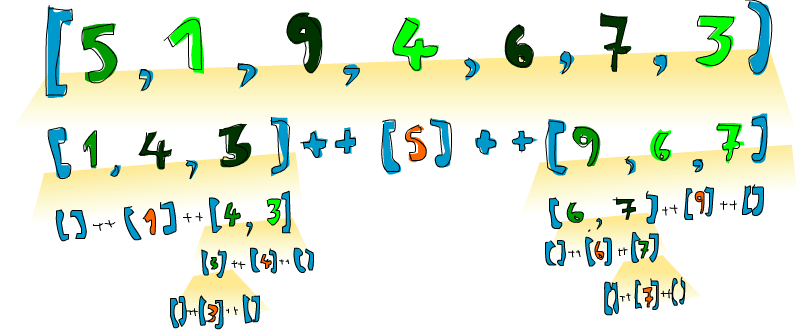
An element that is in place and won’t move anymore is represented in orange. If you read them from left to right, you’ll see the sorted list. Although we chose to compare all the elements to the heads, we could have used any element to compare against. In quicksort, an element that you compare against is called a pivot. They’re in green here. We chose the head because it’s easy to get by pattern matching. The elements that are smaller than the pivot are light green and elements larger than the pivot are dark green. The yellowish gradient thing represents an application of quicksort.

Thinking recursively

We did quite a bit of recursion so far and as you’ve probably noticed, there’s a pattern here. Usually you define an edge case and then you define a function that does something between some element and the function applied to the rest. It doesn’t matter if it’s a list, a tree or any other data structure. A sum is the first element of a list plus the sum of the rest of the list. A product of a list is the first element of the list times the product of the rest of the list. The length of a list is one plus the length of the tail of the list. Et cetera, et cetera…

Of course, these also have edge cases. Usually the edge case is some scenario where a recursive application doesn’t make sense. When dealing with lists, the edge case is most often the empty list. If you’re dealing with trees, the edge case is usually a node that doesn’t have any children.

It’s similar when you’re dealing with numbers recursively. Usually it has to do with some number and the function applied to that number modified. We did the factorial function earlier and it’s the product of a number and the factorial of that number minus one. Such a recursive application doesn’t make sense with zero, because factorials are defined only for positive integers. Often the edge case value turns out to be an identity. The identity for multiplication is 1 because if you multiply something by 1, you get that something back. Also when doing sums of lists, we define the sum of an empty list as 0 and 0 is the identity for addition. In quicksort, the edge case is the empty list and the identity is also the empty list, because if you add an empty list to a list, you just get the original list back.

So when trying to think of a recursive way to solve a problem, try to think of when a recursive solution doesn’t apply and see if you can use that as an edge case, think about identities and think about whether you’ll break apart the parameters of the function (for instance, lists are usually broken into a head and a tail via pattern matching) and on which part you’ll use the recursive call.