Functionally Solving Problems

In this chapter, we’ll take a look at a few interesting problems and how to think functionally to solve them as elegantly as possible. We probably won’t be introducing any new concepts, we’ll just be flexing our newly acquired Haskell muscles and practicing our coding skills. Each section will present a different problem. First we’ll describe the problem, then we’ll try and find out what the best (or least bad) way of solving it is.

Reverse Polish notation calculator

Usually when we write mathematical expressions in school, we write them in an infix manner. For instance, we write 10 - (4 + 3) * 2. +, * and - are infix operators, just like the infix functions we met in Haskell (+, `elem`, etc.). This makes it handy because we, as humans, can parse it easily in our minds by looking at such an expression. The downside to it is that we have to use parentheses to denote precedence.

Reverse Polish notation is another way of writing down mathematical expressions. Initially it looks a bit weird, but it’s actually pretty easy to understand and use because there’s no need for parentheses and it’s very easy to punch into a calculator. While most modern calculators use infix notation, some people still swear by RPN calculators. This is what the previous infix expression looks like in RPN: 10 4 3 + 2 * -. How do we calculate what the result of that is? Well, think of a stack. You go over the expression from left to right. Every time a number is encountered, push it on to the stack. When we encounter an operator, take the two numbers that are on top of the stack (we also say that we pop them), use the operator and those two and then push the resulting number back onto the stack. When you reach the end of the expression, you should be left with a single number if the expression was well-formed and that number represents the result.

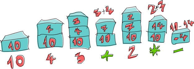
Let’s go over the expression 10 4 3 + 2 * - together! First we push 10 on to the stack and the stack is now 10. The next item is 4, so we push it to the stack as well. The stack is now 10, 4. We do the same with 3 and the stack is now 10, 4, 3. And now, we encounter an operator, namely +! We pop the two top numbers from the stack (so now the stack is just 10), add those numbers together and push that result to the stack. The stack is now 10, 7. We push 2 to the stack, the stack for now is 10, 7, 2. We’ve encountered an operator again, so let’s pop 7 and 2 off the stack, multiply them and push that result to the stack. Multiplying 7 and 2 produces a 14, so the stack we have now is 10, 14. Finally, there’s a -. We pop 10 and 14 from the stack, subtract 14 from 10 and push that back. The number on the stack is now -4 and because there are no more numbers or operators in our expression, that’s our result!

Now that we know how we’d calculate any RPN expression by hand, let’s think about how we could make a Haskell function that takes as its parameter a string that contains a RPN expression, like "10 4 3 + 2 * -" and gives us back its result.

What would the type of that function be? We want it to take a string as a parameter and produce a number as its result. So it will probably be something like solveRPN :: (Num a) => String -> a.

Cool. When implementing a solution to a problem in Haskell, it’s also good to think back on how you did it by hand and maybe try to see if you can gain any insight from that. Here we see that we treated every number or operator that was separated by a space as a single item. So it might help us if we start by breaking a string like "10 4 3 + 2 * -" into a list of items like ["10","4","3","+","2","*","-"].

Next up, what did we do with that list of items in our head? We went over it from left to right and kept a stack as we did that. Does the previous sentence remind you of anything? Remember, in the section about folds, we said that pretty much any function where you traverse a list from left to right or right to left one element by element and build up (accumulate) some result (whether it’s a number, a list, a stack, whatever) can be implemented with a fold.

In this case, we’re going to use a left fold, because we go over the list from left to right. The accumulator value will be our stack and hence, the result from the fold will also be a stack, only as we’ve seen, it will only have one item.

One more thing to think about is, well, how are we going to represent the stack? I propose we use a list. Also I propose that we keep the top of our stack at the head of the list. That’s because adding to the head (beginning) of a list is much faster than adding to the end of it. So if we have a stack of, say, 10, 4, 3, we’ll represent that as the list [3,4,10].

Now we have enough information to roughly sketch our function. It’s going to take a string, like, "10 4 3 + 2 * -" and break it down into a list of items by using words to get ["10","4","3","+","2","*","-"]. Next, we’ll do a left fold over that list and end up with a stack that has a single item, so [-4]. We take that single item out of the list and that’s our final result!

So here’s a sketch of that function:

import Data.List

solveRPN :: (Num a) => String -> a
solveRPN expression = head (foldl foldingFunction [] (words expression))
    where   foldingFunction stack item = ...

We take the expression and turn it into a list of items. Then we fold over that list of items with the folding function. Mind the [], which represents the starting accumulator. The accumulator is our stack, so [] represents an empty stack, which is what we start with. After getting the final stack with a single item, we call head on that list to get the item out and then we apply read.

So all that’s left now is to implement a folding function that will take a stack, like [4,10], and an item, like "3" and return a new stack [3,4,10]. If the stack is [4,10] and the item "*", then it will have to return [40]. But before that, let’s turn our function into point-free style because it has a lot of parentheses that are kind of freaking me out:

import Data.List

solveRPN :: (Num a) => String -> a
solveRPN = head . foldl foldingFunction [] . words
    where   foldingFunction stack item = ...

Ah, there we go. Much better. So, the folding function will take a stack and an item and return a new stack. We’ll use pattern matching to get the top items of a stack and to pattern match against operators like "*" and "-".

solveRPN :: (Num a, Read a) => String -> a
solveRPN = head . foldl foldingFunction [] . words
    where   foldingFunction (x:y:ys) "*" = (x * y):ys
            foldingFunction (x:y:ys) "+" = (x + y):ys
            foldingFunction (x:y:ys) "-" = (y - x):ys
            foldingFunction xs numberString = read numberString:xs

We laid this out as four patterns. The patterns will be tried from top to bottom. First the folding function will see if the current item is "*". If it is, then it will take a list like [3,4,9,3] and call its first two elements x and y respectively. So in this case, x would be 3 and y would be 4. ys would be [9,3]. It will return a list that’s just like ys, only it has x and y multiplied as its head. So with this we pop the two topmost numbers off the stack, multiply them and push the result back on to the stack. If the item is not "*", the pattern matching will fall through and "+" will be checked, and so on.

If the item is none of the operators, then we assume it’s a string that represents a number. If it’s a number, we just call read on that string to get a number from it and return the previous stack but with that number pushed to the top.

And that’s it! Also noticed that we added an extra class constraint of Read a to the function declaration, because we call read on our string to get the number. So this declaration means that the result can be of any type that’s part of the Num and Read typeclasses (like Int, Float, etc.).

For the list of items ["2","3","+"], our function will start folding from the left. The intial stack will be []. It will call the folding function with [] as the stack (accumulator) and "2" as the item. Because that item is not an operator, it will be read and the added to the beginning of []. So the new stack is now [2] and the folding function will be called with [2] as the stack and ["3"] as the item, producing a new stack of [3,2]. Then, it’s called for the third time with [3,2] as the stack and "+" as the item. This causes these two numbers to be popped off the stack, added together and pushed back. The final stack is [5], which is the number that we return.

Let’s play around with our function:

ghci> solveRPN "10 4 3 + 2 * -"
-4
ghci> solveRPN "2 3 +"
5
ghci> solveRPN "90 34 12 33 55 66 + * - +"
-3947
ghci> solveRPN "90 34 12 33 55 66 + * - + -"
4037
ghci> solveRPN "90 34 12 33 55 66 + * - + -"
4037
ghci> solveRPN "90 3 -"
87

Cool, it works! One nice thing about this function is that it can be easily modified to support various other operators. They don’t even have to be binary operators. For instance, we can make an operator "log" that just pops one number off the stack and pushes back its logarithm. We can also make ternary operators that pop three numbers off the stack and push back a result or operators like "sum" which pop off all the numbers and push back their sum.

Let’s modify our function to take a few more operators. For simplicity’s sake, we’ll change its type declaration so that it returns a number of type Float.

import Data.List

solveRPN :: String -> Float
solveRPN = head . foldl foldingFunction [] . words
    where   foldingFunction (x:y:ys) "*" = (x * y):ys
            foldingFunction (x:y:ys) "+" = (x + y):ys
            foldingFunction (x:y:ys) "-" = (y - x):ys
            foldingFunction (x:y:ys) "/" = (y / x):ys
            foldingFunction (x:y:ys) "^" = (y ** x):ys
            foldingFunction (x:xs) "ln" = log x:xs
            foldingFunction xs "sum" = [sum xs]
            foldingFunction xs numberString = read numberString:xs

Wow, great! / is division of course and ** is floating point exponentiation. With the logarithm operator, we just pattern match against a single element and the rest of the stack because we only need one element to perform its natural logarithm. With the sum operator, we just return a stack that has only one element, which is the sum of the stack so far.

ghci> solveRPN "2.7 ln"
0.9932518
ghci> solveRPN "10 10 10 10 sum 4 /"
10.0
ghci> solveRPN "10 10 10 10 10 sum 4 /"
12.5
ghci> solveRPN "10 2 ^"
100.0

Notice that we can include floating point numbers in our expression because read knows how to read them.

ghci> solveRPN "43.2425 0.5 ^"
6.575903

I think that making a function that can calculate arbitrary floating point RPN expressions and has the option to be easily extended in 10 lines is pretty awesome.

One thing to note about this function is that it’s not really fault-tolerant. When given input that doesn’t make sense, it will just crash everything. We’ll make a fault-tolerant version of this with a type declaration of solveRPN :: String -> Maybe Float once we get to know monads (they’re not scary, trust me!). We could make one right now, but it would be a bit tedious because it would involve a lot of checking for Nothing on every step. If you’re feeling up to the challenge though, you can go ahead and try it! Hint: you can use reads to see if a read was successful or not.

Heathrow to London

Our next problem is this: your plane has just landed in England and you rent a car. You have a meeting really soon and you have to get from Heathrow Airport to London as fast as you can (but safely!).

There are two main roads going from Heathrow to London and there’s a number of regional roads crossing them. It takes you a fixed amount of time to travel from one crossroads to another. It’s up to you to find the optimal path to take so that you get to London as fast as you can! You start on the left side and can either cross to the other main road or go forward.

As you can see in the picture, the shortest path from Heathrow to London in this case is to start on main road B, cross over, go forward on A, cross over again and then go forward twice on B. If we take this path, it takes us 75 minutes. Had we chosen any other path, it would take more than that.

Our job is to make a program that takes input that represents a road system and print out what the shortest path across it is. Here’s what the input would look like for this case:

50
10
30
5
90
20
40
2
25
10
8
0

To mentally parse the input file, read it in threes and mentally split the road system into sections. Each section is comprised of a road A, road B and a crossing road. To have it neatly fit into threes, we say that there’s a last crossing section that takes 0 minutes to drive over. That’s because we don’t care where we arrive in London, as long as we’re in London.

Just like we did when solving the RPN calculator problem, we’re going to solve this problem in three steps:

• Forget Haskell for a minute and think about how we’d solve the problem by hand
• Think about how we’re going to represent our data in Haskell
• Figure out how to operate on that data in Haskell so that we produce at a solution

In the RPN calculator section, we first figured out that when calculating an expression by hand, we’d keep a sort of stack in our minds and then go over the expression one item at a time. We decided to use a list of strings to represent our expression. Finally, we used a left fold to walk over the list of strings while keeping a stack to produce a solution.

Okay, so how would we figure out the shortest path from Heathrow to London by hand? Well, we can just sort of look at the whole picture and try to guess what the shortest path is and hopefully we’ll make a guess that’s right. That solution works for very small inputs, but what if we have a road that has 10,000 sections? Yikes! We also won’t be able to say for certain that our solution is the optimal one, we can just sort of say that we’re pretty sure.

That’s not a good solution then. Here’s a simplified picture of our road system:

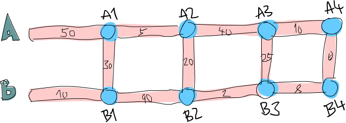
Alright, can you figure out what the shortest path to the first crossroads (the first blue dot on A, marked A1) on road A is? That’s pretty trivial. We just see if it’s shorter to go directly forward on A or if it’s shorter to go forward on B and then cross over. Obviously, it’s cheaper to go forward via B and then cross over because that takes 40 minutes, whereas going directly via A takes 50 minutes. What about crossroads B1? Same thing. We see that it’s a lot cheaper to just go directly via B (incurring a cost of 10 minutes), because going via A and then crossing over would take us a whole 80 minutes!

Now we know what the cheapest path to A1 is (go via B and then cross over, so we’ll say that’s B, C with a cost of 40) and we know what the cheapest path to B1 is (go directly via B, so that’s just B, going at 10). Does this knowledge help us at all if we want to know the cheapest path to the next crossroads on both main roads? Gee golly, it sure does!

Let’s see what the shortest path to A2 would be. To get to A2, we’ll either go directly to A2 from A1 or we’ll go forward from B1 and then cross over (remember, we can only move forward or cross to the other side). And because we know the cost to A1 and B1, we can easily figure out what the best path to A2 is. It costs 40 to get to A1 and then 5 to get from A1 to A2, so that’s B, C, A for a cost of 45. It costs only 10 to get to B1, but then it would take an additional 110 minutes to go to B2 and then cross over! So obviously, the cheapest path to A2 is B, C, A. In the same way, the cheapest way to B2 is to go forward from A1 and then cross over.

Now that we have the best path to A2 and B2, we can repeat this indefinitely until we reach the end. Once we’ve gotten the best paths for A4 and B4, the one that’s cheaper is the optimal path!

So in essence, for the second section, we just repeat the step we did at first, only we take into account what the previous best paths on A and B. We could say that we also took into account the best paths on A and on B in the first step, only they were both empty paths with a cost of 0.

Here’s a summary. To get the best path from Heathrow to London, we do this: first we see what the best path to the next crossroads on main road A is. The two options are going directly forward or starting at the opposite road, going forward and then crossing over. We remember the cost and the path. We use the same method to see what the best path to the next crossroads on main road B is and remember that. Then, we see if the path to the next crossroads on A is cheaper if we go from the previous A crossroads or if we go from the previous B crossroads and then cross over. We remember the cheaper path and then we do the same for the crossroads opposite of it. We do this for every section until we reach the end. Once we’ve reached the end, the cheapest of the two paths that we have is our optimal path!

So in essence, we keep one shortest path on the A road and one shortest path on the B road and when we reach the end, the shorter of those two is our path. We now know how to figure out the shortest path by hand. If you had enough time, paper and pencils, you could figure out the shortest path through a road system with any number of sections.

Next step! How do we represent this road system with Haskell’s data types? One way is to think of the starting points and crossroads as nodes of a graph that point to other crossroads. If we imagine that the starting points actually point to each other with a road that has a length of one, we see that every crossroads (or node) points to the node on the other side and also to the next one on its side. Except for the last nodes, they just point to the other side.

data Node = Node Road Road | EndNode Road
data Road = Road Int Node

A node is either a normal node and has information about the road that leads to the other main road and the road that leads to the next node or an end node, which only has information about the road to the other main road. A road keeps information about how long it is and which node it points to. For instance, the first part of the road on the A main road would be Road 50 a1 where a1 would be a node Node x y, where x and y are roads that point to B1 and A2.

Another way would be to use Maybe for the road parts that point forward. Each node has a road part that point to the opposite road, but only those nodes that aren’t the end ones have road parts that point forward.

data Node = Node Road (Maybe Road)
data Road = Road Int Node

This is an alright way to represent the road system in Haskell and we could certainly solve this problem with it, but maybe we could come up with something simpler? If we think back to our solution by hand, we always just checked the lengths of three road parts at once: the road part on the A road, its opposite part on the B road and part C, which touches those two parts and connects them. When we were looking for the shortest path to A1 and B1, we only had to deal with the lengths of the first three parts, which have lengths of 50, 10 and 30. We’ll call that one section. So the road system that we use for this example can be easily represented as four sections: 50, 10, 30, 5, 90, 20, 40, 2, 25, and 10, 8, 0.

It’s always good to keep our data types as simple as possible, although not any simpler!

data Section = Section { getA :: Int, getB :: Int, getC :: Int } deriving (Show)
type RoadSystem = [Section]

This is pretty much perfect! It’s as simple as it goes and I have a feeling it’ll work perfectly for implementing our solution. Section is a simple algebraic data type that holds three integers for the lengths of its three road parts. We introduce a type synonym as well, saying that RoadSystem is a list of sections.

Our road system from Heathrow to London can now be represented like this:

heathrowToLondon :: RoadSystem
heathrowToLondon = [Section 50 10 30, Section 5 90 20, Section 40 2 25, Section 10 8 0]

All we need to do now is to implement the solution that we came up with previously in Haskell. What should the type declaration for a function that calculates a shortest path for any given road system be? It should take a road system as a parameter and return a path. We’ll represent a path as a list as well. Let’s introduce a Label type that’s just an enumeration of either A, B or C. We’ll also make a type synonym: Path.

data Label = A | B | C deriving (Show)
type Path = [(Label, Int)]

Our function, we’ll call it optimalPath should thus have a type declaration of optimalPath :: RoadSystem -> Path. If called with the road system heathrowToLondon, it should return the following path:

[(B,10),(C,30),(A,5),(C,20),(B,2),(B,8)]

We’re going to have to walk over the list with the sections from left to right and keep the optimal path on A and optimal path on B as we go along. We’ll accumulate the best path as we walk over the list, left to right. What does that sound like? Ding, ding, ding! That’s right, A LEFT FOLD!

When doing the solution by hand, there was a step that we repeated over and over again. It involved checking the optimal paths on A and B so far and the current section to produce the new optimal paths on A and B. For instance, at the beginning the optimal paths were [] and [] for A and B respectively. We examined the section Section 50 10 30 and concluded that the new optimal path to A1 is [(B,10),(C,30)] and the optimal path to B1 is [(B,10)]. If you look at this step as a function, it takes a pair of paths and a section and produces a new pair of paths. The type is (Path, Path) -> Section -> (Path, Path). Let’s go ahead and implement this function, because it’s bound to be useful.

roadStep :: (Path, Path) -> Section -> (Path, Path)
roadStep (pathA, pathB) (Section a b c) =
    let priceA = sum $ map snd pathA
        priceB = sum $ map snd pathB
        forwardPriceToA = priceA + a
        crossPriceToA = priceB + b + c
        forwardPriceToB = priceB + b
        crossPriceToB = priceA + a + c
        newPathToA = if forwardPriceToA <= crossPriceToA
                        then (A,a):pathA
                        else (C,c):(B,b):pathB
        newPathToB = if forwardPriceToB <= crossPriceToB
                        then (B,b):pathB
                        else (C,c):(A,a):pathA
    in  (newPathToA, newPathToB)

What’s going on here? First, calculate the optimal price on road A based on the best so far on A and we do the same for B. We do sum $ map snd pathA, so if pathA is something like [(A,100),(C,20)], priceA becomes 120. forwardPriceToA is the price that we would pay if we went to the next crossroads on A if we went there directly from the previous crossroads on A. It equals the best price to our previous A, plus the length of the A part of the current section. crossPriceToA is the price that we would pay if we went to the next A by going forward from the previous B and then crossing over. It’s the best price to the previous B so far plus the B length of the section plus the C length of the section. We determine forwardPriceToB and crossPriceToB in the same manner.

Now that we know what the best way to A and B is, we just need to make the new paths to A and B based on that. If it’s cheaper to go to A by just going forwards, we set newPathToA to be (A,a):pathA. Basically we prepend the Label A and the section length a to the optimal path path on A so far. Basically, we say that the best path to the next A crossroads is the path to the previous A crossroads and then one section forward via A. Remember, A is just a label, whereas a has a type of Int. Why do we prepend instead of doing pathA ++ [(A,a)]? Well, adding an element to the beginning of a list (also known as consing) is much faster than adding it to the end. This means that the path will be the wrong way around once we fold over a list with this function, but it’s easy to reverse the list later. If it’s cheaper to get to the next A crossroads by going forward from road B and then crossing over, then newPathToA is the old path to B that then goes forward and crosses to A. We do the same thing for newPathToB, only everything’s mirrored.

Finally, we return newPathToA and newPathToB in a pair.

Let’s run this function on the first section of heathrowToLondon. Because it’s the first section, the best paths on A and B parameter will be a pair of empty lists.

ghci> roadStep ([], []) (head heathrowToLondon)
([(C,30),(B,10)],[(B,10)])

Remember, the paths are reversed, so read them from right to left. From this we can read that the best path to the next A is to start on B and then cross over to A and that the best path to the next B is to just go directly forward from the starting point at B.

Now that we have a function that takes a pair of paths and a section and produces a new optimal path, we can just easily do a left fold over a list of sections. roadStep is called with ([],[]) and the first section and returns a pair of optimal paths to that section. Then, it’s called with that pair of paths and the next section and so on. When we’ve walked over all the sections, we’re left with a pair of optimal paths and the shorter of them is our answer. With this in mind, we can implement optimalPath.

optimalPath :: RoadSystem -> Path
optimalPath roadSystem =
    let (bestAPath, bestBPath) = foldl roadStep ([],[]) roadSystem
    in  if sum (map snd bestAPath) <= sum (map snd bestBPath)
            then reverse bestAPath
            else reverse bestBPath

We left fold over roadSystem (remember, it’s a list of sections) with the starting accumulator being a pair of empty paths. The result of that fold is a pair of paths, so we pattern match on the pair to get the paths themselves. Then, we check which one of these was cheaper and return it. Before returning it, we also reverse it, because the optimal paths so far were reversed due to us choosing consing over appending.

Let’s test this!

ghci> optimalPath heathrowToLondon
[(B,10),(C,30),(A,5),(C,20),(B,2),(B,8),(C,0)]

This is the result that we were supposed to get! Awesome! It differs from our expected result a bit because there’s a step (C,0) at the end, which means that we cross over to the other road once we’re in London, but because that crossing doesn’t cost anything, this is still the correct result.

We have the function that finds an optimal path based on, now we just have to read a textual representation of a road system from the standard input, convert it into a type of RoadSystem, run that through our optimalPath function and print the path.

First off, let’s make a function that takes a list and splits it into groups of the same size. We’ll call it groupsOf. For a parameter of [1..10], groupsOf 3 should return [[1,2,3],[4,5,6],[7,8,9],[10]].

groupsOf :: Int -> [a] -> [[a]]
groupsOf 0 _ = undefined
groupsOf _ [] = []
groupsOf n xs = take n xs : groupsOf n (drop n xs)

A standard recursive function. For an xs of [1..10] and an n of 3, this equals [1,2,3] : groupsOf 3 [4,5,6,7,8,9,10]. When the recursion is done, we get our list in groups of three. And here’s our main function, which reads from the standard input, makes a RoadSystem out of it and prints out the shortest path:

import Data.List

main = do
    contents <- getContents
    let threes = groupsOf 3 (map read $ lines contents)
        roadSystem = map (\[a,b,c] -> Section a b c) threes
        path = optimalPath roadSystem
        pathString = concat $ map (show . fst) path
        pathPrice = sum $ map snd path
    putStrLn $ "The best path to take is: " ++ pathString
    putStrLn $ "The price is: " ++ show pathPrice

First, we get all the contents from the standard input. Then, we call lines with our contents to convert something like "50\n10\n30\n... to ["50","10","30".. and then we map read to that to convert it to a list of numbers. We call groupsOf 3 on it so that we turn it to a list of lists of length 3. We map the lambda (\[a,b,c] -> Section a b c) over that list of lists. As you can see, the lambda just takes a list of length 3 and turns it into a section. So roadSystem is now our system of roads and it even has the correct type, namely RoadSystem (or [Section]). We call optimalPath with that and then get the path and the price in a nice textual representation and print it out.

We save the following text

50
10
30
5
90
20
40
2
25
10
8
0

in a file called paths.txt and then feed it to our program.

$ cat paths.txt | runhaskell heathrow.hs
The best path to take is: BCACBBC
The price is: 75

Works like a charm! You can use your knowledge of the Data.Random module to generate a much longer system of roads, which you can then feed to what we just wrote. If you get stack overflows, try using foldl' instead of foldl, because foldl' is strict.