A Fistful of Monads

When we first talked about functors, we saw that they were a useful concept for values that can be mapped over. Then, we took that concept one step further by introducing applicative functors, which allow us to view values of certain data types as values with contexts and use normal functions on those values while preserving the meaning of those contexts.

In this chapter, we’ll learn about monads, which are just beefed up applicative functors, much like applicative functors are only beefed up functors.

When we started off with functors, we saw that it’s possible to map functions over various data types. We saw that for this purpose, the Functor type class was introduced and it had us asking the question: when we have a function of type a -> b and some data type f a, how do we map that function over the data type to end up with f b? We saw how to map something over a Maybe a, a list [a], an IO a etc. We even saw how to map a function a -> b over other functions of type r -> a to get functions of type r -> b. To answer this question of how to map a function over some data type, all we had to do was look at the type of fmap:

fmap :: (Functor f) => (a -> b) -> f a -> f b

And then make it work for our data type by writing the appropriate Functor instance.

Then we saw a possible improvement of functors and said, hey, what if that function a -> b is already wrapped inside a functor value? Like, what if we have Just (*3), how do we apply that to Just 5? What if we don’t want to apply it to Just 5 but to a Nothing instead? Or if we have [(*2),(+4)], how would we apply that to [1,2,3]? How would that work even? For this, the Applicative type class was introduced, in which we wanted the answer to the following type:

(<*>) :: (Applicative f) => f (a -> b) -> f a -> f b

We also saw that we can take a normal value and wrap it inside a data type. For instance, we can take a 1 and wrap it so that it becomes a Just 1. Or we can make it into a [1]. Or an I/O action that does nothing and just yields 1. The function that does this is called pure.

Like we said, an applicative value can be seen as a value with an added context. A fancy value, to put it in technical terms. For instance, the character 'a' is just a normal character, whereas Just 'a' has some added context. Instead of a Char, we have a Maybe Char, which tells us that its value might be a character, but it could also be an absence of a character.

It was neat to see how the Applicative type class allowed us to use normal functions on these values with context and how that context was preserved. Observe:

ghci> (*) <$> Just 2 <*> Just 8
Just 16
ghci> (++) <$> Just "klingon" <*> Nothing
Nothing
ghci> (-) <$> [3,4] <*> [1,2,3]
[2,1,0,3,2,1]

Ah, cool, so now that we treat them as applicative values, Maybe a values represent computations that might have failed, [a] values represent computations that have several results (non-deterministic computations), IO a values represent values that have side-effects, etc.

Monads are a natural extension of applicative functors and with them we’re concerned with this: if you have a value with a context, m a, how do you apply to it a function that takes a normal a and returns a value with a context? That is, how do you apply a function of type a -> m b to a value of type m a? So essentially, we will want this function:

(>>=) :: (Monad m) => m a -> (a -> m b) -> m b

If we have a fancy value and a function that takes a normal value but returns a fancy value, how do we feed that fancy value into the function? This is the main question that we will concern ourselves when dealing with monads. We write m a instead of f a because the m stands for Monad, but monads are just applicative functors that support >>=. The >>= function is pronounced as bind.

When we have a normal value a and a normal function a -> b it’s really easy to feed the value to the function — you just apply the function to the value normally and that’s it. But when we’re dealing with values that come with certain contexts, it takes a bit of thinking to see how these fancy values are fed to functions and how to take into account their behavior, but you’ll see that it’s easy as one two three.

Getting our feet wet with Maybe

Now that we have a vague idea of what monads are about, let’s see if we can make that idea a bit less vague.

Much to no one’s surprise, Maybe is a monad, so let’s explore it a bit more and see if we can combine it with what we know about monads.

A value of type Maybe a represents a value of type a with the context of possible failure attached. A value of Just "dharma" means that the string "dharma" is there whereas a value of Nothing represents its absence, or if you look at the string as the result of a computation, it means that the computation has failed.

When we looked at Maybe as a functor, we saw that if we want to fmap a function over it, it gets mapped over the insides if it’s a Just value, otherwise the Nothing is kept because there’s nothing to map it over!

Like this:

ghci> fmap (++"!") (Just "wisdom")
Just "wisdom!"
ghci> fmap (++"!") Nothing
Nothing

As an applicative functor, it functions similarly. However, applicatives also have the function wrapped. Maybe is an applicative functor in such a way that when we use <*> to apply a function inside a Maybe to a value that’s inside a Maybe, they both have to be Just values for the result to be a Just value, otherwise the result is Nothing. It makes sense because if you’re missing either the function or the thing you’re applying it to, you can’t make something up out of thin air, so you have to propagate the failure:

ghci> Just (+3) <*> Just 3
Just 6
ghci> Nothing <*> Just "greed"
Nothing
ghci> Just ord <*> Nothing
Nothing

When we use the applicative style to have normal functions act on Maybe values, it’s similar. All the values have to be Just values, otherwise it’s all for Nothing!

ghci> max <$> Just 3 <*> Just 6
Just 6
ghci> max <$> Just 3 <*> Nothing
Nothing

And now, let’s think about how we would do >>= for Maybe. Like we said, >>= takes a monadic value, and a function that takes a normal value and returns a monadic value and manages to apply that function to the monadic value. How does it do that, if the function takes a normal value? Well, to do that, it has to take into account the context of that monadic value.

In this case, >>= would take a Maybe a value and a function of type a -> Maybe b and somehow apply the function to the Maybe a. To figure out how it does that, we can use the intuition that we have from Maybe being an applicative functor. Let’s say that we have a function \x -> Just (x+1). It takes a number, adds 1 to it and wraps it in a Just:

ghci> (\x -> Just (x+1)) 1
Just 2
ghci> (\x -> Just (x+1)) 100
Just 101

If we feed it 1, it evaluates to Just 2. If we give it the number 100, the result is Just 101. Very straightforward. Now here’s the kicker: how do we feed a Maybe value to this function? If we think about how Maybe acts as an applicative functor, answering this is pretty easy. If we feed it a Just value, take what’s inside the Just and apply the function to it. If give it a Nothing, hmm, well, then we’re left with a function but Nothing to apply it to. In that case, let’s just do what we did before and say that the result is Nothing.

Instead of calling it >>=, let’s call it applyMaybe for now. It takes a Maybe a and a function that returns a Maybe b and manages to apply that function to the Maybe a. Here it is in code:

applyMaybe :: Maybe a -> (a -> Maybe b) -> Maybe b
applyMaybe Nothing f  = Nothing
applyMaybe (Just x) f = f x

Okay, now let’s play with it for a bit. We’ll use it as an infix function so that the Maybe value is on the left side and the function on the right:

ghci> Just 3 `applyMaybe` \x -> Just (x+1)
Just 4
ghci> Just "smile" `applyMaybe` \x -> Just (x ++ " :)")
Just "smile :)"
ghci> Nothing `applyMaybe` \x -> Just (x+1)
Nothing
ghci> Nothing `applyMaybe` \x -> Just (x ++ " :)")
Nothing

In the above example, we see that when we used applyMaybe with a Just value and a function, the function simply got applied to the value inside the Just. When we tried to use it with a Nothing, the whole result was Nothing. What about if the function returns a Nothing? Let’s see:

ghci> Just 3 `applyMaybe` \x -> if x > 2 then Just x else Nothing
Just 3
ghci> Just 1 `applyMaybe` \x -> if x > 2 then Just x else Nothing
Nothing

Just what we expected. If the monadic value on the left is a Nothing, the whole thing is Nothing. And if the function on the right returns a Nothing, the result is Nothing again. This is very similar to when we used Maybe as an applicative and we got a Nothing result if somewhere in there was a Nothing.

It looks like that for Maybe, we’ve figured out how to take a fancy value and feed it to a function that takes a normal value and returns a fancy one. We did this by keeping in mind that a Maybe value represents a computation that might have failed.

You might be asking yourself, how is this useful? It may seem like applicative functors are stronger than monads, since applicative functors allow us to take a normal function and make it operate on values with contexts. We’ll see that monads can do that as well because they’re an upgrade of applicative functors, and that they can also do some cool stuff that applicative functors can’t.

We’ll come back to Maybe in a minute, but first, let’s check out the type class that belongs to monads.

The Monad type class

Just like functors have the Functor type class and applicative functors have the Applicative type class, monads come with their own type class: Monad! Wow, who would have thought? This is what the type class looks like:

class Monad m where
    return :: a -> m a

    (>>=) :: m a -> (a -> m b) -> m b

    (>>) :: m a -> m b -> m b
    x >> y = x >>= \_ -> y

    fail :: String -> m a
    fail msg = error msg

Let’s start with the first line. It says class Monad m where. But wait, didn’t we say that monads are just beefed up applicative functors? Shouldn’t there be a class constraint in there along the lines of class (Applicative m) = > Monad m where so that a type has to be an applicative functor first before it can be made a monad? Well, there should, but when Haskell was made, it hadn’t occurred to people that applicative functors are a good fit for Haskell so they weren’t in there. But rest assured, every monad is an applicative functor, even if the Monad class declaration doesn’t say so.

The first function that the Monad type class defines is return. It’s the same as pure, only with a different name. Its type is (Monad m) => a -> m a. It takes a value and puts it in a minimal default context that still holds that value. In other words, it takes something and wraps it in a monad. It always does the same thing as the pure function from the Applicative type class, which means we’re already acquainted with return. We already used return when doing I/O. We used it to take a value and make a bogus I/O action that does nothing but yield that value. For Maybe it takes a value and wraps it in a Just.

The next function is >>=, or bind. It’s like function application, only instead of taking a normal value and feeding it to a normal function, it takes a monadic value (that is, a value with a context) and feeds it to a function that takes a normal value but returns a monadic value.

Next up, we have >>. We won’t pay too much attention to it for now because it comes with a default implementation and we pretty much never implement it when making Monad instances.

The final function of the Monad type class is fail. We never use it explicitly in our code. Instead, it’s used by Haskell to enable failure in a special syntactic construct for monads that we’ll meet later. We don’t need to concern ourselves with fail too much for now.

Now that we know what the Monad type class looks like, let’s take a look at how Maybe is an instance of Monad!

instance Monad Maybe where
    return x = Just x
    Nothing >>= f = Nothing
    Just x >>= f  = f x
    fail _ = Nothing

return is the same as pure, so that one’s a no-brainer. We do what we did in the Applicative type class and wrap it in a Just.

The >>= function is the same as our applyMaybe. When feeding the Maybe a to our function, we keep in mind the context and return a Nothing if the value on the left is Nothing because if there’s no value then there’s no way to apply our function to it. If it’s a Just we take what’s inside and apply f to it.

We can play around with Maybe as a monad:

ghci> return "WHAT" :: Maybe String
Just "WHAT"
ghci> Just 9 >>= \x -> return (x*10)
Just 90
ghci> Nothing >>= \x -> return (x*10)
Nothing

Nothing new or exciting on the first line since we already used pure with Maybe and we know that return is just pure with a different name. The next two lines showcase >>= a bit more.

Notice how when we fed Just 9 to the function \x -> return (x*10), the x took on the value 9 inside the function. It seems as though we were able to extract the value from a Maybe without pattern-matching. And we still didn’t lose the context of our Maybe value, because when it’s Nothing, the result of using >>= will be Nothing as well.

Walk the line

Now that we know how to feed a Maybe a value to a function of type a -> Maybe b while taking into account the context of possible failure, let’s see how we can use >>= repeatedly to handle computations of several Maybe a values.

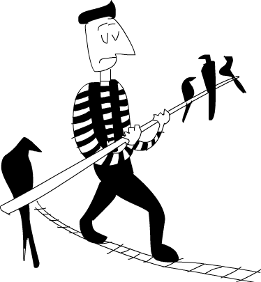
Pierre has decided to take a break from his job at the fish farm and try tightrope walking. He’s not that bad at it, but he does have one problem: birds keep landing on his balancing pole! They come and they take a short rest, chat with their avian friends and then take off in search of breadcrumbs. This wouldn’t bother him so much if the number of birds on the left side of the pole was always equal to the number of birds on the right side. But sometimes, all the birds decide that they like one side better and so they throw him off balance, which results in an embarrassing tumble for Pierre (he’s using a safety net).

Let’s say that he keeps his balance if the number of birds on the left side of the pole and on the right side of the pole is within three. So if there’s one bird on the right side and four birds on the left side, he’s okay. But if a fifth bird lands on the left side, then he loses his balance and takes a dive.

We’re going to simulate birds landing on and flying away from the pole and see if Pierre is still at it after a certain number of birdy arrivals and departures. For instance, we want to see what happens to Pierre if first one bird arrives on the left side, then four birds occupy the right side and then the bird that was on the left side decides to fly away.

We can represent the pole with a simple pair of integers. The first component will signify the number of birds on the left side and the second component the number of birds on the right side:

type Birds = Int
type Pole = (Birds,Birds)

First we made a type synonym for Int, called Birds, because we’re using integers to represent how many birds there are. And then we made a type synonym (Birds,Birds) and we called it Pole (not to be confused with a person of Polish descent).

Next up, how about we make a function that takes a number of birds and lands them on one side of the pole. Here are the functions:

landLeft :: Birds -> Pole -> Pole
landLeft n (left,right) = (left + n,right)

landRight :: Birds -> Pole -> Pole
landRight n (left,right) = (left,right + n)

Pretty straightforward stuff. Let’s try them out:

ghci> landLeft 2 (0,0)
(2,0)
ghci> landRight 1 (1,2)
(1,3)
ghci> landRight (-1) (1,2)
(1,1)

To make birds fly away we just had a negative number of birds land on one side. Because landing a bird on the Pole returns a Pole, we can chain applications of landLeft and landRight:

ghci> landLeft 2 (landRight 1 (landLeft 1 (0,0)))
(3,1)

When we apply the function landLeft 1 to (0,0) we get (1,0). Then, we land a bird on the right side, resulting in (1,1). Finally two birds land on the left side, resulting in (3,1). We apply a function to something by first writing the function and then writing its parameter, but here it would be better if the pole went first and then the landing function. If we make a function like this:

x -: f = f x

We can apply functions by first writing the parameter and then the function:

ghci> 100 -: (*3)
300
ghci> True -: not
False
ghci> (0,0) -: landLeft 2
(2,0)

By using this, we can repeatedly land birds on the pole in a more readable manner:

ghci> (0,0) -: landLeft 1 -: landRight 1 -: landLeft 2
(3,1)

Pretty cool! This example is equivalent to the one before where we repeatedly landed birds on the pole, only it looks neater. Here, it’s more obvious that we start off with (0,0) and then land one bird one the left, then one on the right and finally two on the left.

So far so good, but what happens if 10 birds land on one side?

ghci> landLeft 10 (0,3)
(10,3)

10 birds on the left side and only 3 on the right? That’s sure to send poor Pierre falling through the air! This is pretty obvious here but what if we had a sequence of landings like this:

ghci> (0,0) -: landLeft 1 -: landRight 4 -: landLeft (-1) -: landRight (-2)
(0,2)

It might seem like everything is okay but if you follow the steps here, you’ll see that at one time there are 4 birds on the right side and no birds on the left! To fix this, we have to take another look at our landLeft and landRight functions. From what we’ve seen, we want these functions to be able to fail. That is, we want them to return a new pole if the balance is okay but fail if the birds land in a lopsided manner. And what better way to add a context of failure to value than by using Maybe! Let’s rework these functions:

landLeft :: Birds -> Pole -> Maybe Pole
landLeft n (left,right)
    | abs ((left + n) - right) < 4 = Just (left + n, right)
    | otherwise                    = Nothing

landRight :: Birds -> Pole -> Maybe Pole
landRight n (left,right)
    | abs (left - (right + n)) < 4 = Just (left, right + n)
    | otherwise                    = Nothing

Instead of returning a Pole these functions now return a Maybe Pole. They still take the number of birds and the old pole as before, but then they check if landing that many birds on the pole would throw Pierre off balance. We use guards to check if the difference between the number of birds on the new pole is less than 4. If it is, we wrap the new pole in a Just and return that. If it isn’t, we return a Nothing, indicating failure.

Let’s give these babies a go:

ghci> landLeft 2 (0,0)
Just (2,0)
ghci> landLeft 10 (0,3)
Nothing

Nice! When we land birds without throwing Pierre off balance, we get a new pole wrapped in a Just. But when many more birds end up on one side of the pole, we get a Nothing. This is cool, but we seem to have lost the ability to repeatedly land birds on the pole. We can’t do landLeft 1 (landRight 1 (0,0)) anymore because when we apply landRight 1 to (0,0), we don’t get a Pole, but a Maybe Pole. landLeft 1 takes a Pole and not a Maybe Pole.

We need a way of taking a Maybe Pole and feeding it to a function that takes a Pole and returns a Maybe Pole. Luckily, we have >>=, which does just that for Maybe. Let’s give it a go:

ghci> landRight 1 (0,0) >>= landLeft 2
Just (2,1)

Remember, landLeft 2 has a type of Pole -> Maybe Pole. We couldn’t just feed it the Maybe Pole that is the result of landRight 1 (0,0), so we use >>= to take that value with a context and give it to landLeft 2. >>= does indeed allow us to treat the Maybe value as a value with context because if we feed a Nothing into landLeft 2, the result is Nothing and the failure is propagated:

ghci> Nothing >>= landLeft 2
Nothing

With this, we can now chain landings that may fail because >>= allows us to feed a monadic value to a function that takes a normal one.

Here’s a sequence of birdy landings:

ghci> return (0,0) >>= landRight 2 >>= landLeft 2 >>= landRight 2
Just (2,4)

At the beginning, we used return to take a pole and wrap it in a Just. We could have just applied landRight 2 to (0,0), it would have been the same, but this way we can be more consistent by using >>= for every function. Just (0,0) gets fed to landRight 2, resulting in Just (0,2). This, in turn, gets fed to landLeft 2, resulting in Just (2,2), and so on.

Remember this example from before we introduced failure into Pierre’s routine:

ghci> (0,0) -: landLeft 1 -: landRight 4 -: landLeft (-1) -: landRight (-2)
(0,2)

It didn’t simulate his interaction with birds very well because in the middle there his balance was off but the result didn’t reflect that. But let’s give that a go now by using monadic application (>>=) instead of normal application:

ghci> return (0,0) >>= landLeft 1 >>= landRight 4 >>= landLeft (-1) >>= landRight (-2)
Nothing

Awesome. The final result represents failure, which is what we expected. Let’s see how this result was obtained. First, return puts (0,0) into a default context, making it a Just (0,0). Then, Just (0,0) >>= landLeft 1 happens. Since the Just (0,0) is a Just value, landLeft 1 gets applied to (0,0), resulting in a Just (1,0), because the birds are still relatively balanced. Next, Just (1,0) >>= landRight 4 takes place and the result is Just (1,4) as the balance of the birds is still intact, although just barely. Just (1,4) gets fed to landLeft (-1). This means that landLeft (-1) (1,4) takes place. Now because of how landLeft works, this results in a Nothing, because the resulting pole is off balance. Now that we have a Nothing, it gets fed to landRight (-2), but because it’s a Nothing, the result is automatically Nothing, as we have nothing to apply landRight (-2) to.

We couldn’t have achieved this by just using Maybe as an applicative. If you try it, you’ll get stuck, because applicative functors don’t allow for the applicative values to interact with each other very much. They can, at best, be used as parameters to a function by using the applicative style. The applicative operators will fetch their results and feed them to the function in a manner appropriate for each applicative and then put the final applicative value together, but there isn’t that much interaction going on between them. Here, however, each step relies on the previous one’s result. On every landing, the possible result from the previous one is examined and the pole is checked for balance. This determines whether the landing will succeed or fail.

We may also devise a function that ignores the current number of birds on the balancing pole and just makes Pierre slip and fall. We can call it banana:

banana :: Pole -> Maybe Pole
banana _ = Nothing

Now we can chain it together with our bird landings. It will always cause our walker to fall, because it ignores whatever’s passed to it and always returns a failure. Check it:

ghci> return (0,0) >>= landLeft 1 >>= banana >>= landRight 1
Nothing

The value Just (1,0) gets fed to banana, but it produces a Nothing, which causes everything to result in a Nothing. How unfortunate!

Instead of making functions that ignore their input and just return a predetermined monadic value, we can use the >> function, whose default implementation is this:

(>>) :: (Monad m) => m a -> m b -> m b
m >> n = m >>= \_ -> n

Normally, passing some value to a function that ignores its parameter and always just returns some predetermined value would always result in that predetermined value. With monads however, their context and meaning has to be considered as well. Here’s how >> acts with Maybe:

ghci> Nothing >> Just 3
Nothing
ghci> Just 3 >> Just 4
Just 4
ghci> Just 3 >> Nothing
Nothing

If you replace >> with >>= \_ ->, it’s easy to see why it acts like it does.

We can replace our banana function in the chain with a >> and then a Nothing:

ghci> return (0,0) >>= landLeft 1 >> Nothing >>= landRight 1
Nothing

There we go, guaranteed and obvious failure!

It’s also worth taking a look at what this would look like if we hadn’t made the clever choice of treating Maybe values as values with a failure context and feeding them to functions like we did. Here’s how a series of bird landings would look like:

routine :: Maybe Pole
routine = case landLeft 1 (0,0) of
    Nothing -> Nothing
    Just pole1 -> case landRight 4 pole1 of
        Nothing -> Nothing
        Just pole2 -> case landLeft 2 pole2 of
            Nothing -> Nothing
            Just pole3 -> landLeft 1 pole3

We land a bird on the left and then we examine the possibility of failure and the possibility of success. In the case of failure, we return a Nothing. In the case of success, we land birds on the right and then do the same thing all over again. Converting this monstrosity into a neat chain of monadic applications with >>= is a classic example of how the Maybe monad saves us a lot of time when we have to successively do computations that are based on computations that might have failed.

Notice how the Maybe implementation of >>= features exactly this logic of seeing if a value is Nothing and if it is, returning a Nothing right away and if it isn’t, going forward with what’s inside the Just.

In this section, we took some functions that we had and saw that they would work better if the values that they returned supported failure. By turning those values into Maybe values and replacing normal function application with >>=, we got a mechanism for handling failure pretty much for free, because >>= is supposed to preserve the context of the value to which it applies functions. In this case, the context was that our values were values with failure and so when we applied functions to such values, the possibility of failure was always taken into account.

do notation

Monads in Haskell are so useful that they got their own special syntax called do notation. We’ve already encountered do notation when we were doing I/O and there we said that it was for gluing together several I/O actions into one. Well, as it turns out, do notation isn’t just for IO, but can be used for any monad. Its principle is still the same: gluing together monadic values in sequence. We’re going to take a look at how do notation works and why it’s useful.

Consider this familiar example of monadic application:

ghci> Just 3 >>= (\x -> Just (show x ++ "!"))
Just "3!"

Been there, done that. Feeding a monadic value to a function that returns one, no big deal. Notice how when we do this, x becomes 3 inside the lambda. Once we’re inside that lambda, it’s just a normal value rather than a monadic value. Now, what if we had another >>= inside that function? Check this out:

ghci> Just 3 >>= (\x -> Just "!" >>= (\y -> Just (show x ++ y)))
Just "3!"

Ah, a nested use of >>=! In the outermost lambda, we feed Just "!" to the lambda \y -> Just (show x ++ y). Inside this lambda, the y becomes "!". x is still 3 because we got it from the outer lambda. All this sort of reminds me of the following expression:

ghci> let x = 3; y = "!" in show x ++ y
"3!"

The main difference between these two is that the values in the former example are monadic. They’re values with a failure context. We can replace any of them with a failure:

ghci> Nothing >>= (\x -> Just "!" >>= (\y -> Just (show x ++ y)))
Nothing
ghci> Just 3 >>= (\x -> Nothing >>= (\y -> Just (show x ++ y)))
Nothing
ghci> Just 3 >>= (\x -> Just "!" >>= (\y -> Nothing))
Nothing

In the first line, feeding a Nothing to a function naturally results in a Nothing. In the second line, we feed Just 3 to a function and the x becomes 3, but then we feed a Nothing to the inner lambda and the result of that is Nothing, which causes the outer lambda to produce Nothing as well. So this is sort of like assigning values to variables in let expressions, only that the values in question are monadic values.

To further illustrate this point, let’s write this in a script and have each Maybe value take up its own line:

foo :: Maybe String
foo = Just 3   >>= (\x ->
      Just "!" >>= (\y ->
      Just (show x ++ y)))

To save us from writing all these annoying lambdas, Haskell gives us do notation. It allows us to write the previous piece of code like this:

foo :: Maybe String
foo = do
    x <- Just 3
    y <- Just "!"
    Just (show x ++ y)

It would seem as though we’ve gained the ability to temporarily extract things from Maybe values without having to check if the Maybe values are Just values or Nothing values at every step. How cool! If any of the values that we try to extract from are Nothing, the whole do expression will result in a Nothing. We’re yanking out their (possibly existing) values and letting >>= worry about the context that comes with those values. It’s important to remember that do expressions are just different syntax for chaining monadic values.

In a do expression, every line is a monadic value. To inspect its result, we use <-. If we have a Maybe String and we bind it with <- to a variable, that variable will be a String, just like when we used >>= to feed monadic values to lambdas. The last monadic value in a do expression, like Just (show x ++ y) here, can’t be used with <- to bind its result, because that wouldn’t make sense if we translated the do expression back to a chain of >>= applications. Rather, its result is the result of the whole glued up monadic value, taking into account the possible failure of any of the previous ones.

For instance, examine the following line:

ghci> Just 9 >>= (\x -> Just (x > 8))
Just True

Because the left parameter of >>= is a Just value, the lambda is applied to 9 and the result is a Just True. If we rewrite this in do notation, we get:

marySue :: Maybe Bool
marySue = do
    x <- Just 9
    Just (x > 8)

If we compare these two, it’s easy to see why the result of the whole monadic value is the result of the last monadic value in the do expression with all the previous ones chained into it.

Our tightwalker’s routine can also be expressed with do notation. landLeft and landRight take a number of birds and a pole and produce a pole wrapped in a Just, unless the tightwalker slips, in which case a Nothing is produced. We used >>= to chain successive steps because each one relied on the previous one and each one had an added context of possible failure. Here’s two birds landing on the left side, then two birds landing on the right and then one bird landing on the left:

routine :: Maybe Pole
routine = do
    start <- return (0,0)
    first <- landLeft 2 start
    second <- landRight 2 first
    landLeft 1 second

Let’s see if he succeeds:

ghci> routine
Just (3,2)

He does! Great. When we were doing these routines by explicitly writing >>=, we usually said something like return (0,0) >>= landLeft 2, because landLeft 2 is a function that returns a Maybe value. With do expressions however, each line must feature a monadic value. So we explicitly pass the previous Pole to the landLeft landRight functions. If we examined the variables to which we bound our Maybe values, start would be (0,0), first would be (2,0) and so on.

Because do expressions are written line by line, they may look like imperative code to some people. But the thing is, they’re just sequential, as each value in each line relies on the result of the previous ones, along with their contexts (in this case, whether they succeeded or failed).

Again, let’s take a look at what this piece of code would look like if we hadn’t used the monadic aspects of Maybe:

routine :: Maybe Pole
routine =
    case Just (0,0) of
        Nothing -> Nothing
        Just start -> case landLeft 2 start of
            Nothing -> Nothing
            Just first -> case landRight 2 first of
                Nothing -> Nothing
                Just second -> landLeft 1 second

See how in the case of success, the tuple inside Just (0,0) becomes start, the result of landLeft 2 start becomes first, etc.

If we want to throw the Pierre a banana peel in do notation, we can do the following:

routine :: Maybe Pole
routine = do
    start <- return (0,0)
    first <- landLeft 2 start
    Nothing
    second <- landRight 2 first
    landLeft 1 second

When we write a line in do notation without binding the monadic value with <-, it’s just like putting >> after the monadic value whose result we want to ignore. We sequence the monadic value but we ignore its result because we don’t care what it is and it’s prettier than writing _ <- Nothing, which is equivalent to the above.

When to use do notation and when to explicitly use >>= is up to you. I think this example lends itself to explicitly writing >>= because each step relies specifically on the result of the previous one. With do notation, we had to specifically write on which pole the birds are landing, but every time we used that came directly before. But still, it gave us some insight into do notation.

In do notation, when we bind monadic values to names, we can utilize pattern matching, just like in let expressions and function parameters. Here’s an example of pattern matching in a do expression:

justH :: Maybe Char
justH = do
    (x:xs) <- Just "hello"
    return x

We use pattern matching to get the first character of the string "hello" and then we present it as the result. So justH evaluates to Just 'h'.

What if this pattern matching were to fail? When matching on a pattern in a function fails, the next pattern is matched. If the matching falls through all the patterns for a given function, an error is thrown and our program crashes. On the other hand, failed pattern matching in let expressions results in an error being produced right away, because the mechanism of falling through patterns isn’t present in let expressions. When pattern matching fails in a do expression, the fail function is called. It’s part of the Monad type class and it enables failed pattern matching to result in a failure in the context of the current monad instead of making our program crash. Its default implementation is this:

fail :: (Monad m) => String -> m a
fail msg = error msg

So by default it does make our program crash, but monads that incorporate a context of possible failure (like Maybe) usually implement it on their own. For Maybe, its implemented like so:

fail _ = Nothing

It ignores the error message and makes a Nothing. So when pattern matching fails in a Maybe value that’s written in do notation, the whole value results in a Nothing. This is preferable to having our program crash. Here’s a do expression with a pattern that’s bound to fail:

wopwop :: Maybe Char
wopwop = do
    (x:xs) <- Just ""
    return x

The pattern matching fails, so the effect is the same as if the whole line with the pattern was replaced with a Nothing. Let’s try this out:

ghci> wopwop
Nothing

The failed pattern matching has caused a failure within the context of our monad instead of causing a program-wide failure, which is pretty neat.

The list monad

So far, we’ve seen how Maybe values can be viewed as values with a failure context and how we can incorporate failure handling into our code by using >>= to feed them to functions. In this section, we’re going to take a look at how to use the monadic aspects of lists to bring non-determinism into our code in a clear and readable manner.

We’ve already talked about how lists represent non-deterministic values when they’re used as applicatives. A value like 5 is deterministic. It has only one result and we know exactly what it is. On the other hand, a value like [3,8,9] contains several results, so we can view it as one value that is actually many values at the same time. Using lists as applicative functors showcases this non-determinism nicely:

ghci> (*) <$> [1,2,3] <*> [10,100,1000]
[10,100,1000,20,200,2000,30,300,3000]

All the possible combinations of multiplying elements from the left list with elements from the right list are included in the resulting list. When dealing with non-determinism, there are many choices that we can make, so we just try all of them, and so the result is a non-deterministic value as well, only it has many more results.

This context of non-determinism translates to monads very nicely. Let’s go ahead and see what the Monad instance for lists looks like:

instance Monad [] where
    return x = [x]
    xs >>= f = concat (map f xs)
    fail _ = []

return does the same thing as pure, so we should already be familiar with return for lists. It takes a value and puts it in a minimal default context that still yields that value. In other words, it makes a list that has only that one value as its result. This is useful for when we want to just wrap a normal value into a list so that it can interact with non-deterministic values.

To understand how >>= works for lists, it’s best if we take a look at it in action to gain some intuition first. >>= is about taking a value with a context (a monadic value) and feeding it to a function that takes a normal value and returns one that has context. If that function just produced a normal value instead of one with a context, >>= wouldn’t be so useful because after one use, the context would be lost. Anyway, let’s try feeding a non-deterministic value to a function:

ghci> [3,4,5] >>= \x -> [x,-x]
[3,-3,4,-4,5,-5]

When we used >>= with Maybe, the monadic value was fed into the function while taking care of possible failures. Here, it takes care of non-determinism for us. [3,4,5] is a non-deterministic value and we feed it into a function that returns a non-deterministic value as well. The result is also non-deterministic, and it features all the possible results of taking elements from the list [3,4,5] and passing them to the function \x -> [x,-x]. This function takes a number and produces two results: one negated and one that’s unchanged. So when we use >>= to feed this list to the function, every number is negated and also kept unchanged. The x from the lambda takes on every value from the list that’s fed to it.

To see how this is achieved, we can just follow the implementation. First, we start off with the list [3,4,5]. Then, we map the lambda over it and the result is the following:

[[3,-3],[4,-4],[5,-5]]

The lambda is applied to every element and we get a list of lists. Finally, we just flatten the list and voila! We’ve applied a non-deterministic function to a non-deterministic value!

Non-determinism also includes support for failure. The empty list [] is pretty much the equivalent of Nothing, because it signifies the absence of a result. That’s why failing is just defined as the empty list. The error message gets thrown away. Let’s play around with lists that fail:

ghci> [] >>= \x -> ["bad","mad","rad"]
[]
ghci> [1,2,3] >>= \x -> []
[]

In the first line, an empty list is fed into the lambda. Because the list has no elements, none of them can be passed to the function and so the result is an empty list. This is similar to feeding Nothing to a function. In the second line, each element gets passed to the function, but the element is ignored and the function just returns an empty list. Because the function fails for every element that goes in it, the result is a failure.

Just like with Maybe values, we can chain several lists with >>=, propagating the non-determinism:

ghci> [1,2] >>= \n -> ['a','b'] >>= \ch -> return (n,ch)
[(1,'a'),(1,'b'),(2,'a'),(2,'b')]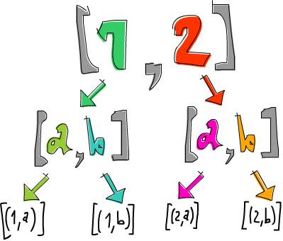

The list [1,2] gets bound to n and ['a','b'] gets bound to ch. Then, we do return (n,ch) (or [(n,ch)]), which means taking a pair of (n,ch) and putting it in a default minimal context. In this case, it’s making the smallest possible list that still presents (n,ch) as the result and features as little non-determinism as possible. Its effect on the context is minimal. What we’re saying here is this: for every element in [1,2], go over every element in ['a','b'] and produce a tuple of one element from each list.

Generally speaking, because return takes a value and wraps it in a minimal context, it doesn’t have any extra effect (like failing in Maybe or resulting in more non-determinism for lists) but it does present something as its result.

Here’s the previous expression rewritten in do notation:

listOfTuples :: [(Int,Char)]
listOfTuples = do
    n <- [1,2]
    ch <- ['a','b']
    return (n,ch)

This makes it a bit more obvious that n takes on every value from [1,2] and ch takes on every value from ['a','b']. Just like with Maybe, we’re extracting the elements from the monadic values and treating them like normal values and >>= takes care of the context for us. The context in this case is non-determinism.

Using lists with do notation really reminds me of something we’ve seen before. Check out the following piece of code:

ghci> [ (n,ch) | n <- [1,2], ch <- ['a','b'] ]
[(1,'a'),(1,'b'),(2,'a'),(2,'b')]

Yes! List comprehensions! In our do notation example, n became every result from [1,2] and for every such result, ch was assigned a result from ['a','b'] and then the final line put (n,ch) into a default context (a singleton list) to present it as the result without introducing any additional non-determinism. In this list comprehension, the same thing happened, only we didn’t have to write return at the end to present (n,ch) as the result because the output part of a list comprehension did that for us.

In fact, list comprehensions are just syntactic sugar for using lists as monads. In the end, list comprehensions and lists in do notation translate to using >>= to do computations that feature non-determinism.

List comprehensions allow us to filter our output. For instance, we can filter a list of numbers to search only for that numbers whose digits contain a 7:

ghci> [ x | x <- [1..50], '7' `elem` show x ]
[7,17,27,37,47]

We apply show to x to turn our number into a string and then we check if the character '7' is part of that string. Pretty clever. To see how filtering in list comprehensions translates to the list monad, we have to check out the guard function and the MonadPlus type class. The MonadPlus type class is for monads that can also act as monoids. Here’s its definition:

class Monad m => MonadPlus m where
    mzero :: m a
    mplus :: m a -> m a -> m a

mzero is synonymous to mempty from the Monoid type class and mplus corresponds to mappend. Because lists are monoids as well as monads, they can be made an instance of this type class:

instance MonadPlus [] where
    mzero = []
    mplus = (++)

For lists mzero represents a non-deterministic computation that has no results at all — a failed computation. mplus joins two non-deterministic values into one. The guard function is defined like this:

guard :: (MonadPlus m) => Bool -> m ()
guard True = return ()
guard False = mzero

It takes a boolean value and if it’s True, takes a () and puts it in a minimal default context that still succeeds. Otherwise, it makes a failed monadic value. Here it is in action:

ghci> guard (5 > 2) :: Maybe ()
Just ()
ghci> guard (1 > 2) :: Maybe ()
Nothing
ghci> guard (5 > 2) :: [()]
[()]
ghci> guard (1 > 2) :: [()]
[]

Looks interesting, but how is it useful? In the list monad, we use it to filter out non-deterministic computations. Observe:

ghci> [1..50] >>= (\x -> guard ('7' `elem` show x) >> return x)
[7,17,27,37,47]

The result here is the same as the result of our previous list comprehension. How does guard achieve this? Let’s first see how guard functions in conjunction with >>:

ghci> guard (5 > 2) >> return "cool" :: [String]
["cool"]
ghci> guard (1 > 2) >> return "cool" :: [String]
[]

If guard succeeds, the result contained within it is an empty tuple. So then, we use >> to ignore that empty tuple and present something else as the result. However, if guard fails, then so will the return later on, because feeding an empty list to a function with >>= always results in an empty list. A guard basically says: if this boolean is False then produce a failure right here, otherwise make a successful value that has a dummy result of () inside it. All this does is to allow the computation to continue.

Here’s the previous example rewritten in do notation:

sevensOnly :: [Int]
sevensOnly = do
    x <- [1..50]
    guard ('7' `elem` show x)
    return x

Had we forgotten to present x as the final result by using return, the resulting list would just be a list of empty tuples. Here’s this again in the form of a list comprehension:

ghci> [ x | x <- [1..50], '7' `elem` show x ]
[7,17,27,37,47]

So filtering in list comprehensions is the same as using guard.

A knight’s quest

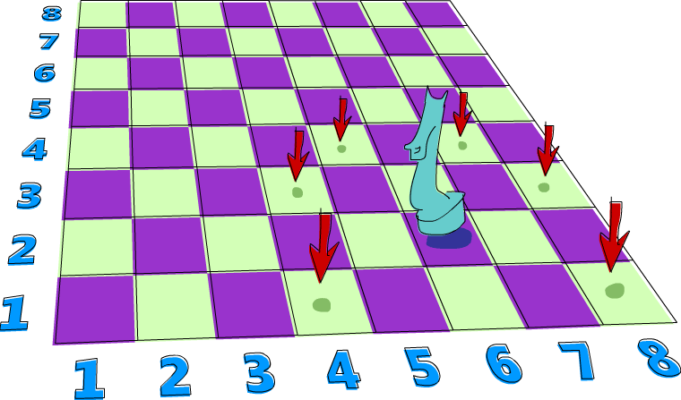
Here’s a problem that really lends itself to being solved with non-determinism. Say you have a chess board and only one knight piece on it. We want to find out if the knight can reach a certain position in three moves. We’ll just use a pair of numbers to represent the knight’s position on the chess board. The first number will determine the column he’s in and the second number will determine the row.

Let’s make a type synonym for the knight’s current position on the chess board:

type KnightPos = (Int,Int)

So let’s say that the knight starts at (6,2). Can he get to (6,1) in exactly three moves? Let’s see. If we start off at (6,2) what’s the best move to make next? I know, how about all of them! We have non-determinism at our disposal, so instead of picking one move, let’s just pick all of them at once. Here’s a function that takes the knight’s position and returns all of its next moves:

moveKnight :: KnightPos -> [KnightPos]
moveKnight (c,r) = do
    (c',r') <- [(c+2,r-1),(c+2,r+1),(c-2,r-1),(c-2,r+1)
               ,(c+1,r-2),(c+1,r+2),(c-1,r-2),(c-1,r+2)
               ]
    guard (c' `elem` [1..8] && r' `elem` [1..8])
    return (c',r')

The knight can always take one step horizontally or vertically and two steps horizontally or vertically but its movement has to be both horizontal and vertical. (c',r') takes on every value from the list of movements and then guard makes sure that the new move, (c',r') is still on the board. If it it’s not, it produces an empty list, which causes a failure and return (c',r') isn’t carried out for that position.

This function can also be written without the use of lists as a monad, but we did it here just for kicks. Here is the same function done with filter:

moveKnight :: KnightPos -> [KnightPos]
moveKnight (c,r) = filter onBoard
    [(c+2,r-1),(c+2,r+1),(c-2,r-1),(c-2,r+1)
    ,(c+1,r-2),(c+1,r+2),(c-1,r-2),(c-1,r+2)
    ]
    where onBoard (c,r) = c `elem` [1..8] && r `elem` [1..8]

Both of these do the same thing, so pick one that you think looks nicer. Let’s give it a whirl:

ghci> moveKnight (6,2)
[(8,1),(8,3),(4,1),(4,3),(7,4),(5,4)]
ghci> moveKnight (8,1)
[(6,2),(7,3)]

Works like a charm! We take one position and we just carry out all the possible moves at once, so to speak. So now that we have a non-deterministic next position, we just use >>= to feed it to moveKnight. Here’s a function that takes a position and returns all the positions that you can reach from it in three moves:

in3 :: KnightPos -> [KnightPos]
in3 start = do
    first <- moveKnight start
    second <- moveKnight first
    moveKnight second

If you pass it (6,2), the resulting list is quite big, because if there are several ways to reach some position in three moves, it crops up in the list several times. The above without do notation:

in3 start = return start >>= moveKnight >>= moveKnight >>= moveKnight

Using >>= once gives us all possible moves from the start and then when we use >>= the second time, for every possible first move, every possible next move is computed, and the same goes for the last move.

Putting a value in a default context by applying return to it and then feeding it to a function with >>= is the same as just normally applying the function to that value, but we did it here anyway for style.

Now, let’s make a function that takes two positions and tells us if you can get from one to the other in exactly three steps:

canReachIn3 :: KnightPos -> KnightPos -> Bool
canReachIn3 start end = end `elem` in3 start

We generate all the possible positions in three steps and then we see if the position we’re looking for is among them. So let’s see if we can get from (6,2) to (6,1) in three moves:

ghci> (6,2) `canReachIn3` (6,1)
True

Yes! How about from (6,2) to (7,3)?

ghci> (6,2) `canReachIn3` (7,3)
False

No! As an exercise, you can change this function so that when you can reach one position from the other, it tells you which moves to take. Later on, we’ll see how to modify this function so that we also pass it the number of moves to take instead of that number being hardcoded like it is now.

Monad laws

Just like applicative functors, and functors before them, monads come with a few laws that all monad instances must abide by. Just because something is made an instance of the Monad type class doesn’t mean that it’s a monad, it just means that it was made an instance of a type class. For a type to truly be a monad, the monad laws must hold for that type. These laws allow us to make reasonable assumptions about the type and its behavior.

Haskell allows any type to be an instance of any type class as long as the types check out. It can’t check if the monad laws hold for a type though, so if we’re making a new instance of the Monad type class, we have to be reasonably sure that all is well with the monad laws for that type. We can rely on the types that come with the standard library to satisfy the laws, but later when we go about making our own monads, we’re going to have to manually check the if the laws hold. But don’t worry, they’re not complicated.

Left identity

The first monad law states that if we take a value, put it in a default context with return and then feed it to a function by using >>=, it’s the same as just taking the value and applying the function to it. To put it formally:

• return x >>= f is the same damn thing as f x

If you look at monadic values as values with a context and return as taking a value and putting it in a default minimal context that still presents that value as its result, it makes sense, because if that context is really minimal, feeding this monadic value to a function shouldn’t be much different than just applying the function to the normal value, and indeed it isn’t different at all.

For the Maybe monad return is defined as Just. The Maybe monad is all about possible failure, and if we have a value and want to put it in such a context, it makes sense that we treat it as a successful computation because, well, we know what the value is. Here’s some return usage with Maybe:

ghci> return 3 >>= (\x -> Just (x+100000))
Just 100003
ghci> (\x -> Just (x+100000)) 3
Just 100003

For the list monad return puts something in a singleton list. The >>= implementation for lists goes over all the values in the list and applies the function to them, but since there’s only one value in a singleton list, it’s the same as applying the function to that value:

ghci> return "WoM" >>= (\x -> [x,x,x])
["WoM","WoM","WoM"]
ghci> (\x -> [x,x,x]) "WoM"
["WoM","WoM","WoM"]

We said that for IO, using return makes an I/O action that has no side-effects but just presents a value as its result. So it makes sense that this law holds for IO as well.

Right identity

The second law states that if we have a monadic value and we use >>= to feed it to return, the result is our original monadic value. Formally:

• m >>= return is no different than just m

This one might be a bit less obvious than the first one, but let’s take a look at why it should hold. When we feed monadic values to functions by using >>=, those functions take normal values and return monadic ones. return is also one such function, if you consider its type. Like we said, return puts a value in a minimal context that still presents that value as its result. This means that, for instance, for Maybe, it doesn’t introduce any failure and for lists, it doesn’t introduce any extra non-determinism. Here’s a test run for a few monads:

ghci> Just "move on up" >>= (\x -> return x)
Just "move on up"
ghci> [1,2,3,4] >>= (\x -> return x)
[1,2,3,4]
ghci> putStrLn "Wah!" >>= (\x -> return x)
Wah!

If we take a closer look at the list example, the implementation for >>= is:

xs >>= f = concat (map f xs)

So when we feed [1,2,3,4] to return, first return gets mapped over [1,2,3,4], resulting in [[1],[2],[3],[4]] and then this gets concatenated and we have our original list.

Left identity and right identity are basically laws that describe how return should behave. It’s an important function for making normal values into monadic ones and it wouldn’t be good if the monadic value that it produced did a lot of other stuff.

Associativity

The final monad law says that when we have a chain of monadic function applications with >>=, it shouldn’t matter how they’re nested. Formally written:

• Doing (m >>= f) >>= g is just like doing m >>= (\x -> f x >>= g)

Hmmm, now what’s going on here? We have one monadic value, m and two monadic functions f and g. When we’re doing (m >>= f) >>= g, we’re feeding m to f, which results in a monadic value. Then, we feed that monadic value to g. In the expression m >>= (\x -> f x >>= g), we take a monadic value and we feed it to a function that feeds the result of f x to g. It’s not easy to see how those two are equal, so let’s take a look at an example that makes this equality a bit clearer.

Remember when we had our tightrope walker Pierre walk a rope while birds landed on his balancing pole? To simulate birds landing on his balancing pole, we made a chain of several functions that might produce failure:

ghci> return (0,0) >>= landRight 2 >>= landLeft 2 >>= landRight 2
Just (2,4)

We started with Just (0,0) and then bound that value to the next monadic function, landRight 2. The result of that was another monadic value which got bound into the next monadic function, and so on. If we were to explicitly parenthesize this, we’d write:

ghci> ((return (0,0) >>= landRight 2) >>= landLeft 2) >>= landRight 2
Just (2,4)

But we can also write the routine like this:

return (0,0) >>= (\x ->
landRight 2 x >>= (\y ->
landLeft 2 y >>= (\z ->
landRight 2 z)))

return (0,0) is the same as Just (0,0) and when we feed it to the lambda, the x becomes (0,0). landRight takes a number of birds and a pole (a tuple of numbers) and that’s what it gets passed. This results in a Just (0,2) and when we feed this to the next lambda, y is (0,2). This goes on until the final bird landing produces a Just (2,4), which is indeed the result of the whole expression.

So it doesn’t matter how you nest feeding values to monadic functions, what matters is their meaning. Here’s another way to look at this law: consider composing two functions, f and g. Composing two functions is implemented like so:

(.) :: (b -> c) -> (a -> b) -> (a -> c)
f . g = (\x -> f (g x))

If the type of g is a -> b and the type of f is b -> c, we arrange them into a new function which has a type of a -> c, so that its parameter is passed between those functions. Now what if those two functions were monadic, that is, what if the values they returned were monadic values? If we had a function of type a -> m b, we couldn’t just pass its result to a function of type b -> m c, because that function accepts a normal b, not a monadic one. We could however, use >>= to make that happen. So by using >>=, we can compose two monadic functions:

(<=<) :: (Monad m) => (b -> m c) -> (a -> m b) -> (a -> m c)
f <=< g = (\x -> g x >>= f)

So now we can compose two monadic functions:

ghci> let f x = [x,-x]
ghci> let g x = [x*3,x*2]
ghci> let h = f <=< g
ghci> h 3
[9,-9,6,-6]

Cool. So what does that have to do with the associativity law? Well, when we look at the law as a law of compositions, it states that f <=< (g <=< h) should be the same as (f <=< g) <=< h. This is just another way of saying that for monads, the nesting of operations shouldn’t matter.

If we translate the first two laws to use <=<, then the left identity law states that for every monadic function f, f <=< return is the same as writing just f and the right identity law says that return <=< f is also no different from f.

This is very similar to how if f is a normal function, (f . g) . h is the same as f . (g . h), f . id is always the same as f and id . f is also just f.

In this chapter, we took a look at the basics of monads and learned how the Maybe monad and the list monad work. In the next chapter, we’ll take a look at a whole bunch of other cool monads and we’ll also learn how to make our own.